Should you have to isolate data in Google Sheets base on specific criteria in a cell? Well, you can use conditional formatting to highlight entire rows in your spreadsheet. Read on to learn how.
First off, launch your browser and then go to Google Sheets.
Next up, open up a spreadsheet with a table of data which you wish to apply conditional formatting to highlight specific rows.
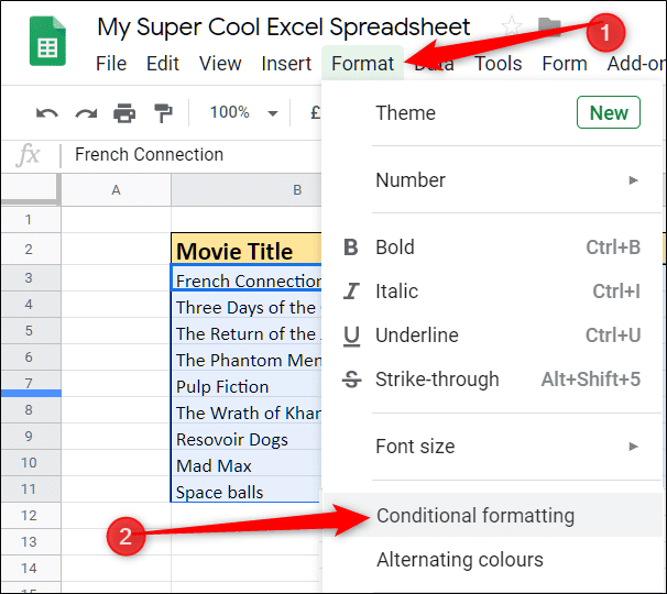
Now, you need to highlight the cells inside the table and then click Format.
From the toolbar that appears, click “Conditional Formatting.”
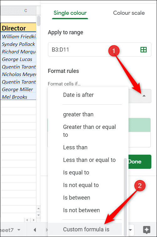
A panel will appear on the right. Click the drop-down menu under “Format Cells If.”
Now, click “Custom Formula Is.”
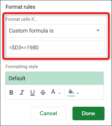
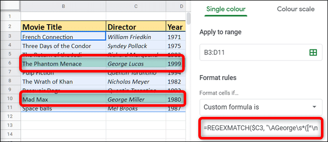
In the “Value or Formula” text box that appears, enter the formula to highlight the specific data you wish to be isolated in the table. In this guide, we will use a formula that highlights an entire row if the release year is before 1980. It looks like this- =$D3<1980.
Now, enter the formula you want to use to search for data. Also, make sure to use the dollar sign before the column letter. This will ensure that the formula only parses the column specified.
What the first part of the formula (=$D3) does is to tell Sheets that we want to start examining the data from cell D3. The dollar sign at the beginning is important, and it says that column (D) is fixed, but the row (3) is flexible. This will enable the formula to check the data in the entire column.
The second part of the formula (>1980) describes the condition the data has to meet to return to True. The example we used helps us to look for movies released before 1980.
Note- If you want your result to include the date entered, use “<=1980.” This will give you a result, including everything released in 1980 as well.
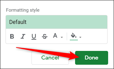
Next up, you need to choose the type of formatting you wish to be applied when the conditions are met. Formatting options include bold, italic, underline, strikethrough, font color, or cell color, and they can all be applied to your results. By default, when results are gotten, the rows are filled with a light-green color.
When you have selected you you want the rows to be displayed after a match has been found, click Done. You can close the panel or create another rule to apply conditional formatting to as well.
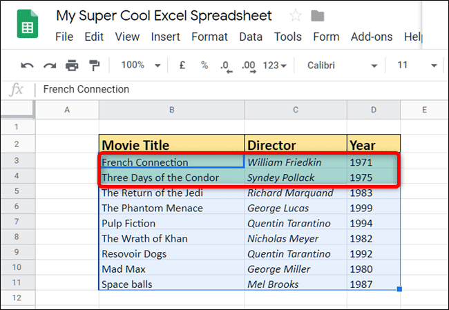
Now, the rows of movies released before 1980 are highlighted in green.
Although the formula used in this guide is a rather simple one, you can use this really helpful tool limitlessly. Even advanced formulas and functions can be used to match data in the table.
That’s it! This tool is perfect for helping you create intricate spreadsheets with beautifully formatted data that catches everyone’s attention.
